

邮箱:zhaoyu_yep@163.com
目录
3. Stata 实操:plssem 命令
4. 参考文献
5. 相关推文
温馨提示: 文中链接在微信中无法生效。请点击底部「阅读原文」。或直接长按/扫描如下二维码,直达原文:
1. 简介
本文拟介绍基于偏最小二乘法的 SEM (PLS-SEM) 的 plssem 命令。该命令是由 Venturini and Mehmetoglu (2019) 编写。与传统统计方法(如线性回归,多元回归等)不同,在更广泛的意义上, SEM 可以作为一个联立多方程的估计模型,在方程的两边可以包括单项或/和多项变量,并有助于对非常复杂的模型进行适当而完整的中介效应分析。在文献中,目前存在着许多关于基于协方差的 SEM(COV-SEM)和 PLS-SEM 优缺点的争论 (如 Henseler et al., 2014), PLS-SEM 通常被认为是一种与 COV-SEM 的互补方法 (Jöreskog, 1969; Wold, 1975)。根据 Hair et al. (2017) 的建议,一般在以下情况下使用 PLS-SEM :
文献详情:
Venturini, S., M. Mehmetoglu, 2019, Plssem: A stata package for structural equation modeling with partial least squares, Journal of Statistical Software, 88 (8): 1-35. -Link-, -PDF-
2. PLS-SEM 方法
一个典型的 PLS-SEM 模型将由两部分组成:测量模型 (measurement) 和 结构模型 (structural),如图 1 所示。

测量模型 (measurement model) 提供了潜在变量和它们所定义的指标之间的关系。由图 1 除虚线框中包含的箭头以外的所有箭头表示。图中包括了两个反射结构( 和 )和一个构成结构()。反射结构/构成结构与相应指标之间的关系由箭头上的系数表示。
结构模型 (structural mode) 显示了潜在变量之间的关系,图 1 中是由虚线框中包含的箭头表示。结构模型中作为预测变量的潜在变量为外生变量,而表示为结果变量的则为内生变量。在图 1 中有两个外生变量( 和 )和一个内生变量(),利用相应的路径系数( 和 )标记潜在变量之间的关系。
用于估计 PLS-SEM 模型的算法基本上由三个阶段组成:
更多的细节参照文献 Venturini and Mehmetoglu (2019)。
2.1 PLS-SEM 的应用情况
在 微软学术 中检索如下经典教材,引用率超过 20000 次:
2.2 PLS-SEM 软件和资源
Get to Know PLS-SEM and SmartPLS 有关 PLS-SEM 的资源汇总
3. Stata 实操:plssem 命令3.1. 命令安装
. ssc install plssem, replace

. help plssem
作者也提供了一些两份范例 dofile 和一个数据文件 workout2.dta (后文会用到)sem结构方程模型是什么,可以用如下命令获取:
. net get plssem.pkg, replace

copying into current directory...
      copying  workout2.dta
      copying  ecsimobi.dta
      copying  plssem_application.do
ancillary files successfully copied.
3.2. 语法结构
. plssem  (LV1 > indblock1)
          (LV2 > indblock2) (...)
          [if] [in]
          [, structural(LV2 LV1, ...) options]
其中,options 包括:
Options描述
wscheme(centroid)
使用质心加权方案
wscheme(factorial)
使用阶乘加权方案
wscheme(path)
使用路径加权方案;默认值
binary(namelist)
使用 logit 匹配的潜在变量列表
boot(numlist)
bootstrap 次数
seed(numlist)
bootstrap 种子数
tol(#)
公差默认值为
maxiter(#)
最大迭代次数;默认值为 100
missing(mean)
使用可用指标的平均值来插补指标缺失值
missing(knn)
用 k 近邻法估算指标缺失值
k(#)
用于 missing(knn)的最近邻数;默认值为 5
init(eigen)
使用因子初始化潜在变量
init(indsum)
使用指标之和初始化潜在变量;默认值
digits(#)
显示的位数;默认值为 3
noheader
禁止显示输出标题
nomeastable
禁止显示判别有效性表
nostructtable
禁止显示结构模型估算表
loadpval
显示外部荷载的 p 值
stats
打印指标的汇总统计表
group()
执行多组分析;有关详细信息,请参见选项
correlate()
报告指标、潜在变量和交叉负荷之间的相关性;有关详细信息,请参见选项
rawsum
将潜在得分估计为指标的原始和
noscale
清单变量在运行算法之前没有标准化
convcrit(relative)
相对收敛准则;默认值
convcrit(square)
平方收敛准则
3.3. Stata 实操
基于相关的进化心理学文献 (如 Kirsner, Figueredo and Jacobs,2003),我们提出以下假设:
根据上述假设,建立如图 2 的关系:
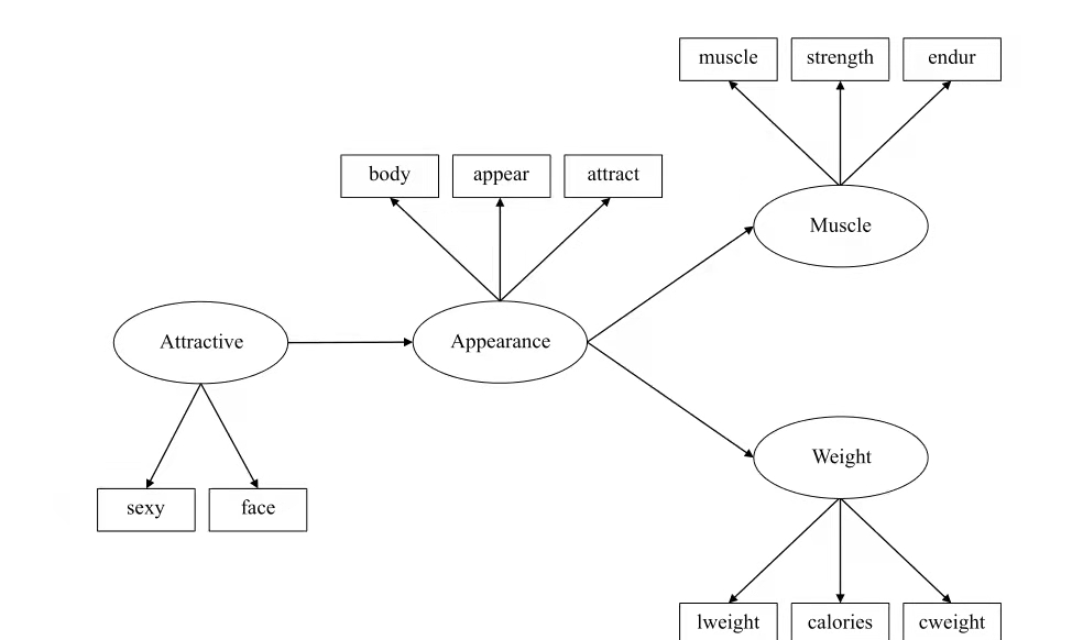
按照第 3.2 节中描述的语法和选项,我们用以下代码指定和估计图 2 中所示的研究模型:
. net get plssem.pkg, replace // 下载数据文件

. use workout2.dta,clear

. plssem (Attractive > face sexy)             ///
         (Appearance > body appear attract)   ///
         (Muscle > muscle strength endur)     ///
         (Weight > lweight calories cweight)  ///
         , ///
         structural(Appearance Attractive, ///
                    Muscle Appearance,     ///
                    Weight Appearance)     ///
         boot(200) seed(123) stats correlate(lv)

. estat indirect, effects(Muscle Appearance Attractive, ///
                          Weight Appearance Attractive) ///
        boot(200) seed(456)

. plssemplot, loadings
. ereturn list
上面的代码行产生以下结果:
. use workout2.dta,clear

. plssem (Attractive > face sexy)             ///
         (Appearance > body appear attract)   ///
         (Muscle > muscle strength endur)     ///
         (Weight > lweight calories cweight)  ///
         , ///
         structural(Appearance Attractive, ///
                    Muscle Appearance,     ///
                    Weight Appearance)     ///
         boot(200) seed(123) stats correlate(lv)

PLS-SEM --> Bootstrap replications (200)
----+--- 1 ---+--- 2 ---+--- 3 ---+--- 4 ---+--- 5
..................................................    50
..................................................   100
..................................................   150
..................................................   200

Iteration 1: outer weights rel. diff. = 6.31e-01
Iteration 2: outer weights rel. diff. = 1.49e-02
Iteration 3: outer weights rel. diff. = 1.34e-03
Iteration 4: outer weights rel. diff. = 7.76e-05
Iteration 5: outer weights rel. diff. = 6.80e-06
Iteration 6: outer weights rel. diff. = 4.00e-07
Iteration 7: outer weights rel. diff. = 3.49e-08

Partial least squares SEM            Number of obs       =  187
                                     Average R-squared   =  0.15795
                                     Average communality =  0.79165
Weighting scheme: path               Absolute GoF        =  0.35361
Tolerance: 1.00e-07                  Relative GoF        =  0.83138
Initialization: indsum               Average redundancy  =  0.11941

Table of summary statistics for indicator variables
-------------------------------------------------------------------
Indicator |   mean      sd   median     min     max     N  missing
----------+--------------------------------------------------------
     face |  3.290   1.005    3.000   1.000   6.000   200       46
     sexy |  2.592   1.113    3.000   1.000   6.000   196       50
     body |  4.034   1.470    4.000   1.000   6.000   205       41
   appear |  3.365   1.672    3.000   1.000   6.000   203       43
  attract |  3.059   1.707    3.000   1.000   6.000   204       42
   muscle |  3.853   1.587    4.000   1.000   6.000   204       42
 strength |  4.779   1.159    5.000   1.000   6.000   208       38
    endur |  4.976   1.111    5.000   1.000   6.000   209       37
  lweight |  3.604   1.759    4.000   1.000   6.000   207       39
 calories |  4.053   1.638    4.000   1.000   6.000   207       39
  cweight |  4.048   1.666    4.000   1.000   6.000   207       39
-------------------------------------------------------------------

Measurement model - Standardized loadings
-------------------------------------------------------------------
          |  Reflective:   Reflective:   Reflective:   Reflective:
          |   Attractive    Appearance        Muscle        Weight
----------+--------------------------------------------------------
     face |        0.908
     sexy |        0.919
     body |                      0.899
   appear |                      0.949
  attract |                      0.923
   muscle |                                    0.886
 strength |                                    0.873
    endur |                                    0.623
  lweight |                                                  0.916
 calories |                                                  0.937
  cweight |                                                  0.911
----------+--------------------------------------------------------
 Cronbach |        0.801         0.914         0.734         0.912
       DG |        0.909         0.946         0.842         0.944
    rho_A |        0.803         0.917         0.849         0.931
-------------------------------------------------------------------

Discriminant validity - Squared interfactor correlation vs. Average variance extracted (AVE)
-----------------------------------------------------------
           |  Attractive   Appearance     Muscle    Weight
-----------+-----------------------------------------------
Attractive |       1.000        0.080      0.021     0.002
Appearance |       0.080        1.000      0.217     0.177
    Muscle |       0.021        0.217      1.000     0.041
    Weight |       0.002        0.177      0.041     1.000
-----------+-----------------------------------------------
       AVE |       0.834        0.854      0.645     0.849
-----------------------------------------------------------

Structural model - Standardized path coefficients (Bootstrap)
-----------------------------------------------------------
     Variable |   Appearance         Muscle         Weight
--------------+--------------------------------------------
   Attractive |        0.283
              |      (0.000)
   Appearance |                       0.466          0.420
              |                     (0.000)        (0.000)
--------------+--------------------------------------------
         r2_a |        0.075          0.213          0.172
-----------------------------------------------------------
 p-values in parentheses

Correlation of latent variables
--------------------------------------------------
             | Attrac~e Appear~e   Muscle   Weight
-------------+------------------------------------
  Attractive |   1.0000
  Appearance |   0.2830   1.0000
      Muscle |   0.1435   0.4658   1.0000
      Weight |  -0.0414   0.4204   0.2032   1.0000
--------------------------------------------------
可以看到,输出以一些汇总统计数据开始,然后是估计结果的测量部分,包括引导标准加载。然后,我们看到一个表,显示了鉴别有效性评估,然后显示了包括自助标准化路径系数在内的估计结果的结构部分。最后,我们得到一个表格,显示了我们的模型潜在变量之间的相关性。
提供的输出为我们提供了测试前三个假设的必要信息,即 、 和 。为了能够检验中介假设( 和 )sem结构方程模型是什么,我们进一步使用以下代码来估计间接效应,并使用bootstrap方法检验其统计显著性。
. estat indirect, effects(Muscle Appearance Attractive, ///
                          Weight Appearance Attractive) ///
        boot(200) seed(456)
Bootstrapping indirect effects...

Significance testing of (standardized) indirect effects (Bootstrap)
--------------------------------------------------------------
                        |        Muscle <- |        Weight <-
 Statistics             |    Appearance <- |    Appearance <-
                        |       Attractive |       Attractive
------------------------+------------------+------------------
 Indirect effect        |            0.132 |            0.119
 Standard error         |            0.040 |            0.033
 Z statistic            |            3.285 |            3.564
 P-value                |            0.001 |            0.000
 Conf. interval (N)     |   (0.053, 0.210) |   (0.054, 0.184)
 Conf. interval (P)     |   (0.066, 0.228) |   (0.067, 0.197)
 Conf. interval (BC)    |   (0.071, 0.240) |   (0.068, 0.198)
--------------------------------------------------------------
 confidence level: 95%
 (N)    normal confidence interval
 (P)    percentile confidence interval
 (BC)   bias-corrected confidence interval
我们可以使用下面的代码进一步要求一个显示每个潜在变量外部负载大小的图形输出,这将产生如图 3 所示的图:
.
. plssemplot, loadings

Loadings
------------------------------------------------------------------
          | Reflective:   Reflective:   Reflective:   Reflective:
          |  Attractive    Appearance        Muscle        Weight
----------+-------------------------------------------------------
     face |      0.9077
     sexy |      0.9186
     body |                    0.8989
   appear |                    0.9492
  attract |                    0.9230
   muscle |                                  0.8856
 strength |                                  0.8730
    endur |                                  0.6225
  lweight |                                                0.9156
 calories |                                                0.9366
  cweight |                                                0.9111
------------------------------------------------------------------
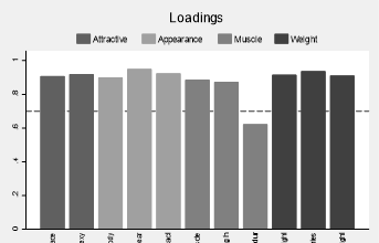
图 3: 外部负载的条形图报告
4. 参考文献
5. 相关推文
Note:产生如下推文列表的 Stata 命令为:
lianxh 结构方程
安装最新版 lianxh 命令:
ssc install lianxh, replace
New! Stata 搜索神器:lianxh 和 songbl
搜: 推文、数据分享、期刊论文、重现代码 ……
安装:
. ssc install lianxh
. ssc install songbl
使用:
. lianxh DID 倍分法
. songbl all
关于我们

限 时 特 惠:本站每日持续更新海量各大内部创业教程,一年会员只需98元,会员全站资源免费获取点击查看会员权益
站 长 微 信:ryenlii666
